
I have been criticized in the past by some of you after earlier lectures to this group. Apparently some people think I tend to get too mathematical and abstruse. Well I’m happy to say that this year will be no different. I am going to subtitle this lecture, “Music, Mathematics, Magnetism, and the Columbus Landfall.” And I’ve brought an audio-visual aid. What does a guitar have to do with Columbus? Hang on, we’ll get there eventually.
When you pluck the string in the center, you get a tone, called a fundamental tone (see Fig. 1).
 |
| Figure 1. Fundamental Wave. |
|---|
If you constrain the center of the string from moving, you get a different tone, one octave higher. This tone is called the first harmonic (Fig. 2). There is also a second harmonic, and a third, and so on, for as high as you want to go.
 |
| Figure 2. First harmonic wave. |
|---|
If you add together some of these harmonics, you get a repeating wave that looks disordered and chaotic (Fig. 3). Although it’s easy to create chaos out of order, one of the neat things about math is, sometimes you can also create order out of chaos. In particular, it has been shown that any wave that repeats itself, no matter how chaotic or random-looking, can be broken down into a set of simple fundamental components. This process of finding the simple components from a complex wave is called harmonic analysis, or Fourier analysis after the mathematician who invented it.
 |
| Figure 3. Adding Harmonics. |
|---|
One way to insure that a wave repeats itself is to wrap it around a circle, as in figure 4. Here, the black line represents the axis, now wrapped in a circle. It’s easy to see that any wave that can be wrapped around a circle like this will always repeat as it meets itself.
 |
| Figure 4. The first harmonic, wrapped around a circle. |
|---|
But it’s even more useful to take our one-dimensional wave and make it two-dimensional, like the waves on the surface of a pond. Then, instead of wrapping the wave around a circle, we can wrap our wave it around a sphere, like figure 5, to insure that it will always repeat. Spherical waves also have component harmonics. And like one-dimensional waves, any spherical wave, no matter how chaotic or random-looking, can be broken down into its simple fundamental components. This process is called spherical harmonic analysis, or SHA.
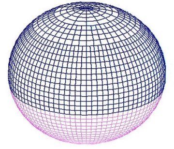 | |
| Figure 5. A simple spherical wave: Degree 1, order 0. |
|---|
As it turns out, a lot of interesting physical phenomena can be modeled with spherical waves. Like the small variations in the earth’s gravitational field, for instance. Or, more to the point, the variations of the earth’s magnetic field.
If the earth’s magnetic field were a perfect dipole – that is, a perfect bar magnet perfectly aligned with the axis of the earth – the spherical wave representing it would look like figure 5, and every compass would always point true north. Since the magnetic field is not a perfect dipole, the direction of the compass does not point exactly north in most times and places; it is usually a few degrees off, one way or another. The difference between true north and magnetic north is called magnetic declination, and as we will see, declination plays a crucial role as we try to trace the route of Columbus across the Atlantic.
This simple wave in figure 5, representing the dipole, comprises 90% of the earth’s magnetic field. It’s the other 10% that’s troublesome. If we want to model the magnetic field using spherical waves, we have to add small parts of a lot of other waves to the model.
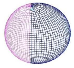
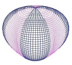
This dipole wave is called a first-order wave. As we continue to add higher-order spherical waves (Figure 6), each successive wave generally adds less and less information to the final model – or, we might say that successive waves tend to have smaller amplitudes. Most of the information in the model lies within the first few orders. For the last twenty years or so, geophysicists have used this technique to develop a standard model of the earth’s current magnetic field. This model, called the International Geomagnetic Reference Field, or IGRF, is a tenth-order model, composed of 120 spherical waves. The IGRF has been shown to predict magnetic declination to within a half-degree of accuracy over oceanic areas – even over those areas too remote to be easily visited.
 |
 |
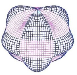 |
| Figure 6. Higher order spherical waves. | ||
|---|---|---|
The earth’s magnetic field changes slowly over time and magnetic declination changes with time too, over periods of several decades. Every five years, the IGRF is updated to reflect these changes. We can map magnetic declination with a chart, called an isogonic chart. An isogon is a line that connects points of equal magnetic declination. Figure 7 is an isogonic chart derived from the IGRF for the year 2000.
 |
| Figure 7. Isongonic chart from the IGRF for year 2000. |
|---|
Having learned that SHA is an efficient way of modeling the geomagnetic field, scientists began to apply the same technique to historical magnetic observations, eventually developing models going back as far as the seventeenth century. Before then, the number of magnetic observations is too sparse for accurate modeling. This is a pity, because if we could model the earth’s magnetic field for the year 1492, we could (in theory) determine the landfall of Columbus by following the magnetic compass courses laid down in his log. We could correct his stated compass courses for magnetic declination to find the true course sailed on each day, starting from the Canary Islands and going all the way across the Atlantic to the Bahamas.
This effort to determine the landfall by tracing the transatlantic track has already been tried at least six times before, but each of these attempts has shortcomings of various types – some of which are quite serious. For example, some simulations determined the currents for the voyage by examining the current arrows drawn on pilot charts of the North Atlantic, a dubious practice at best.
In the open sea, far from the land, ocean currents behave a lot like winds in the atmosphere. Like winds, currents have a prevailing direction, in which they can be expected to move. And like winds, the actual direction experienced on any particular day might be quite different from, or even opposite to, the prevailing direction. This is because daily current direction is dominated by medium-scale structures called mesoeddies, which, like large high and low pressure systems in the atmosphere, form, move, and die over periods of several weeks. (You can see some of them on Figure 8.) Further, there is a seasonal component to the formation of these eddies and currents. Therefore it is impossible to determine the actual currents that Columbus’s fleet experienced in 1492.
 |
| Figure 8. Radar altimetry showing highs and lows on ocean surface. |
|---|
But there are ways of getting close. Doug Peck of SHD made a vast improvement on the practice of eyeballing pilot charts, by actually sailing across the Atlantic in his boat, the Gooney Bird – thus subjecting himself, and his simulation, to the actual currents in that region of the sea.
But certainly the most important shortcoming of all transatlantic track work to date has been our lack of any firm knowledge of the magnetic declination in the North Atlantic at the time of Columbus.
In 1995, I developed a web site devoted to the navigation of Columbus, and to the problem of determining the location of his first landfall in the New World. When I wrote about this issue of tracing the transatlantic track, I proposed that any such tracing, to be scientifically acceptable, should meet the following criteria:
When I proposed these criteria in 1995, I had my doubts that any such scientifically valid study could be done. At the time, there were no SHA models of the magnetic field for the 15th century, and there appeared to be no hope of getting any. Historical geomagnetic observations simply do not go that far back.
Today, after more than ten years of working on this problem, and literally hundreds of computer simulations of transatlantic crossings, I am pleased to say that at last I can meet all of these criteria.
Over the past 20 years, new techniques for determining the magnetic field in historical times have emerged, based not on historical data, but on archaeomagnetic data. When a fire burns over a hearthstone, the heat softens the stone’s grip on tiny magnetic regions within the rock, allowing them to rotate in response to the local magnetic field. When the site is abandoned, the cold rock retains the magnetic alignment of the last time it was heated. Such hearthstones can be dated by conventional archaeological methods, and they can be used as markers for the magnetic field at those particular times and places.
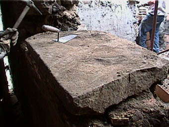 | |
| Archaeomagnetic sources 1: Hearthstones |
|---|
Volcanic eruptions often trap the remains of organic material, such as trees, within lava. If the eruption is recent (in geologic terms), the date of the eruption can be determined using Carbon-14. As the lava cools and solidifies, tiny magnetic regions within the lava solidify in the direction of the magnetic field at the time of the eruption.
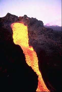 | |
| Archaeomagnetic sources 2: volcanic eruptions |
|---|
In the spring, melting water flows into temperate lakes, bringing a load of silt. Usually, some of these particles are composed of ferrous minerals, and therefore have tiny magnetic regions within them. As the silt particles slowly descend to the bottom, these magnetic regions align themselves with the local magnetic field. When this year’s silt becomes trapped underneath successive layers, their alignments are preserved. Such annual deposits are called varves, and they can be dated by Carbon-14 from organic material within the same layer. Lake varve deposits can provide a continuous record of magnetic field alignments for several millennia in some locations.
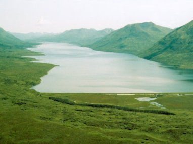 |
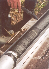 |
| Archaeomagnetic sources 3: lake varves | |
|---|---|
Pile up enough hearthstones, enough volcanic eruptions, and enough lake varves from enough epochs and in enough places around the world, and you can create a magnetic model.
In recent years, several such models have been created. In 1998, Hongre, Hulot, and Khokhlov published a third-order SHA model based on an archaeomagnetic dataset that relied primarily on hearthstone data. Like any third-order model, it was crude, but even a crude model is better than nothing. This model confirmed that magnetic declination at the time of Columbus was easterly in western Europe, and westerly in the north Atlantic.
 |
| Isogonic chart from the Hongre model. |
|---|
 |
| Isogonic chart from the Constable model. |
|---|
Two years later, Constable, Johnson and Lund published another third-order magnetic model for historical times. This model was based on a different archaeomagnetic dataset, drawn primarily from lake varves. It confirmed the westerly declination in the north Atlantic, but the magnitude of this declination was considerably different from the earlier model of Hongre.
It also turns out that neither of these models was capable of meeting the criteria that I had laid out in 1995. The Hongre model was not able to replicate the first voyage eastbound, while the Constable model was not able to re-create the second voyage westbound.
When I first proposed giving this talk some months ago, I thought I would have to stop here, and tell you that progress was being made, but that there were still problems to overcome. However, over the past few years there has been an explosion of newly published lake varve data from all over the world. And at the end of last year a new SHA model of the magnetic field in historical times, using this new data, was published by Korte and Constable in late 2003.
Korte calls her model the Continuous Archaeomagnetic and Lake Sediment model for 3000 years, or CALS3K for short (see Figure 9). This new model takes it data from many more sites and epochs than anything that has come before. Unlike earlier attempts, CALS3K is a full 10th order model of the magnetic field, like the modern IGRF.
 |
| Figure 9. Isogonic chart from the CALS3K model. |
|---|
How accurate is the CALS3K model? As a tenth-order model, the spatial detail is as good as one could wish; but we cannot expect that CALS3K will be as accurate as the IGRF, since the archaeomagnetic data that underlie CALS3K are generally considered accurate to only about 2 degrees or so. Nevertheless, it is possible that at some epochs and in some places, it might approach the half-degree accuracy of the modern IGRF. To know whether it does or not during the time of Columbus and in the North Atlantic, we will have to test the model. In fact, we will use the same tests that I proposed in 1995: the two transatlantic crossings made by Columbus in the year 1493.
When we simulate an ocean voyage, it is very important to keep track of the errors inherent in the process. By far, the largest source of error is the drift of the ship due to the variability of ocean currents. If Doug were to retrace Columbus’s voyage in the Gooney Bird a dozen different times, he would come out at a dozen different locations. Would these locations be clustered tightly, or scattered widely? How can that be determined with confidence? Well, we could cross the ocean a dozen times to find out. But we don’t have to. The Atlantic has already been crossed, not merely dozens of times, but thousands of times, by skilled navigators who have kept careful track of their daily positions. And those records still exist.
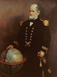 |
| Matthew Fontaine Maury |
|---|
In the 1850’s, Matthew Fontaine Maury (1806-1873), remembered today as the US Navy’s first oceanographer, began collecting daily drift reports from American and Dutch navigators. Every day at noon, a nineteenth-century navigator would shoot the sun to give him his true position. He would then compare his true position to his dead-reckoning position, as computed by the ship’s course and speed sailed from the previous day’s noon fix. The difference in the two positions, if any, is due mostly to the set of the current – although the ship’s leeway also plays a part.
Up until 1975, the US Navy, and later the National Oceanographic and Atmospheric Administration, kept a running collection of this ship drift data, eventually growing to comprise some comprise four million daily drift observations, about half of them taken in the North Atlantic. These are available on CD-ROM. In order to compute the expected current drift at any position, I take all observations that are within one degree of the position in both latitude and longitude. To insure that I do not neglect the seasonality of currents, I also look only at observations within thirty days of the desired date regardless of year. This gives me a subset of observations for this specific location and time of year. The subset contains between several dozen and several hundred individual ship drift observations.
These individual observations are averaged, and the variance of the observations is determined both on the north-south axis and the east-west axis.
 |
| Figure 10. One hour's computation. |
|---|
Here’s how a typical computation works (see Figure 10). In my simulations, I re-computed Columbus’s position for every hour of the voyage. Starting with the stated magnetic course and speed, as given in the log, I compute the magnetic declination at each hourly position according to the CALS3K model, to determine the true course sailed. Then I move the ship along the true course for its known speed. Finally I compute the currents and apply one hour’s worth of average drift for this date and location, while retaining the variances of the drift for later use. Then I repeat the whole process for the next hour, with the new starting position.
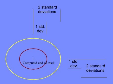 | |
| Figure 11. The error ellipse. |
|---|
At the end of the voyage, we have two results: a final position, and a sum of all the current variances for the voyage (Figure 11). From the current variances we can compute the standard deviation of the current drift on both the north-south axis and the east-west axis. Because of the variability of currents, we cannot claim that the computed final position is exactly where one would end up if such a voyage were actually sailed. The best we can claim is that one would end up near the final position, and we can draw an error ellipse around the final position that shows the standard deviation that we determined from the variance of the currents. If the magnetic model is correct, it is quite likely that any actually sailed voyage would end up within, or pretty close to, this error ellipse.
To validate Korte’s model, the CALS3K model of the magnetic field, let us now look at Columbus’s second voyage westbound, which, he told us, was sailed on a constant west-by-south magnetic course from Hierro in the Canary Islands. Since we do not have a log for this voyage, we have no idea of the speeds sailed on each day; therefore, we must assume a constant average speed adequate for the fleet to arrive at Dominica in the West Indies after a remarkably fast twenty-one day crossing. Figure 12 is the computed end of the transatlantic track using the CALS3K magnetic model. The black cross is the known landfall of Columbus on the second voyage. We know that the landfall was at this point, because Diego Alvarez Chanca tells us, in a letter written after the voyage, that Dominica was the first island seen on the morning of November 3, 1493, and shortly thereafter the island of Guadeloupe was seen. This specific order of seeing these islands as they rise above the horizon can only occur in a very small patch of the ocean, marked here.
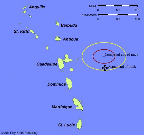 | |
| Figure 12. Endpoint of second voyage, using CALS3K model. |
|---|
Let me say that after ten years of trying probably dozens of isogonic charts as the basis for such simulated voyages, it is extremely gratifying to see that the CALS3K model actually gets to the Dominica landfall. Of all the voyages, this second voyage westbound is in my experience by far the simulation most likely to fail.
Note also that the final computed position is a little to the north of the actual landfall. If we wanted to tinker with the model, we might be tempted to crank in a little extra westerly declination at this point. Since westerly declination draws you leftward regardless of your direction of travel, doing that would make the computed final position fit the actual landfall better. But as we shall see, there is a very good reason for not engaging in such tinkering – even beyond the obvious one of invalidating the science behind the model.
For our next validation test, let’s look at the eastbound passage of Columbus’s first voyage. In this case, we are blessed with the log of the first voyage, which records the actual courses and speeds sailed on each day. Following the same procedure, we can compute the end of the simulated voyage and hope that it arrives at the Azores, as Columbus did on February 15, 1493. And in fact, it does, within the known limits of current variability (see Figure 13). The first thing to notice is that the error ellipse is larger than it was for the voyage to Dominica. This is because this voyage passes through the middle of the North Atlantic gyre, a region of the sea long known for its fickle winds and unpredictable currents. Accordingly, our computed current variances are rather large, and the error ellipse reflects this.
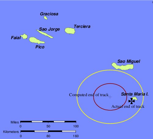 | |
| Figure 13. Endpoint of first voyage eastbound, using CALS3K. |
|---|
Note that here again, the computed final position is a bit to the north of the actual landfall at Santa Maria Island. Here again we are tempted to tinker with the model, to make the computed position fit the actual landfall better. But now, on an eastbound voyage, we would have to crank in more easterly variation to take the final position closer to the actual landfall. But wait a moment. If we add more easterly variation to the model, this final position moves south, but the previous final position, off Domenica, moves north. In other words, the only way to improve the final position on this voyage is to make the final position of the other voyage worse. And conversely, the only way to improve the final position on the Dominica voyage is to make this final position worse.
In a nutshell, because these two voyages were sailed in opposite directions, there is a dynamic tension between them. In my experience, it has been extraordinarily rare to find any magnetic model that can successfully re-create both of these voyages at the same time. That the CALS3K model of Korte & Constable has done this, is a stunning achievement and a tribute to 21st century science.
Finally, this magnetic model is not only successful, it is also strongly constrained. If the average magnetic declination in the North Atlantic at this epoch were different from the model by even half a degree, one way or another, one of these two validation tests would fail. The actual average magnetic declination in the North Atlantic at the time of Columbus must have been very, very close to the CALS3K model prediction.
Having validated the model, and having shown that the model is strongly constrained, naturally we want to know what the model predicts for the first voyage westbound. Can we, at long last, determine the location of the first landfall of Columbus in the New World? The model prediction is shown in Figure 14.
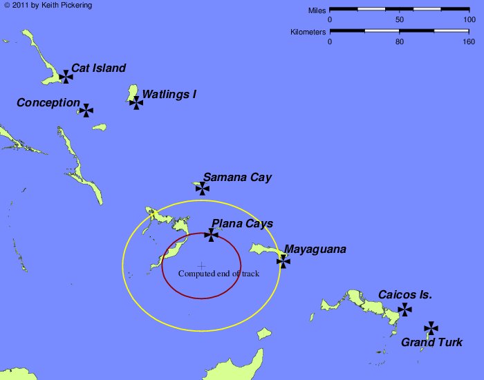 |
| Figure 14. Endpoint of first voyage westbound, using CALS3K. |
|---|
Those of you who were at the 1997 annual meeting might recall that in my lecture that year, I showed through multiple lines of evidence that there were some 32 leagues missing from the log of Columbus in the westbound passage. I also showed where the missing leagues were hiding, and how they might be restored. In my simulation here, I have included those missing leagues. If I had not done so, the center of the error ellipse would have ended up just north of North Caicos Island, and Caicos would have been the only landfall island within the ellipse, although Mayaguana would have been a marginal case.
The black crosses show eight of the ten landfall islands that have been proposed by various theorists over the past two centuries. Given the variability of currents, it is not surprising that we cannot pin down the landfall to a single island on this basis alone. But although we may not be able to say where the landfall is, we can say with some confidence where the landfall isn’t. Grand Turk was the favored landfall for much of the 19th century, and Watlings Island was the favored landfall for much of the 20th century. Twenty-first century science has now rendered both of these theories obsolete.
Samana Cay, the National Geographic’s favored island, lies just outside the error ellipse, yet close enough that I don’t think we can say that it can be eliminated on this basis. The two landfalls inside the error ellipse are Mayaguana, a theory that has never quite caught on for reasons that I can’t fathom (since I’ve always thought it could make a pretty good theory), and closest of all, the Plana Cays, a landfall first proposed by Ramon Didiez Burgos in 1974, and independently by myself in 1994.
I must say from a personal perspective that I find this quite gratifying. Ten years ago, I examined the courses and distances Columbus sailed through the Bahamas. On that basis, the so-called inter-island track, I showed that the Plana Cays had, by far, the best inter-island track of all proposed landfalls. Today I can also say that Plana has the best transatlantic track of all proposed landfalls. For these reasons, I feel completely justified in saying that from a scientific perspective, the Columbus landfall debate is probably over. The CALS3K model has very likely pounded the final nail in the dispute. At this point, there is simply no other theory that fits so much of the evidence so completely as the Plana Cays, Columbus’s first landfall in the New World.
References
Constable, C.G., Johnson, C.L. & Lund, S.P., "Global Geomagnetic Field Models for the Past 3000 Years: Transient or Permanent Flux Lobes?", Philosophical Transactions of the Royal Society of London, ser. A., 358 (2000), 991-1008.
Hongre, L., Hulot, G. & Khokhlov, A., “An Analysis of the Geomagnetic Field over the Past 2000 Years”, Physics of the Earth and Planetary Interiors, 106 (1998), 311-335.
Korte, M., & Constable, C., “Continuous global geomagnetic field models for the past 3000 years,” Physics of the Earth and Planetary Interiors, 140 (2003), 73-89. Data and fortran source code available at http://mahi.ucsd.edu/cathy/Holocene/CALS3K/
National
Geophysical Data Center. GEOMAG (source code to convert SHA coefficients to
magnetic declinations), and the current IGRF model.
http://www.ngdc.noaa.gov/seg/geom_util/utilities_home.shtml.
National Oceanographic Data Center. Ship Drift Surface Currents. CD-ROM available from http://www.nodc.noaa.gov/General/NODC-cdrom.html#oceandrft.
Pickering, Keith A. (1994). Columbus's Plana Landfall. Dio 4:1, 14-23. http://www.dioi.org/vols/w41.pdf
Pickering, Keith A. (1997). The Navigational Mysteries and Fraudulent Longitudes of Christopher Columbus. Lecture given to the Society for the History of Discoveries and the Haklyut Society, August 1997. http://www.columbusnavigation.com/shd973.shtml
Starting position
Sep  8   28.0000  -17.0000     0.00

Day   leg   Lat      Lon    Crs    Lgs  NS-set EW-set  NS-var  EW-var   Mag

Sep  8 1  27.9590 -17.4957 270.00  9.00 -164.1 -304.1    73.5    73.3  -2.63
Sep  9 1  27.9003 -18.4318 270.00 18.00 -195.4 -201.5   148.8   145.4  -3.04
Sep  9 2  28.1088 -20.2666 281.50 36.00 -143.4 -255.6   148.8   145.4  -3.85
Sep 10 1  27.8634 -23.3582 270.00 60.00 -168.6 -168.3   197.2   230.8  -5.16
Sep 11 1  27.7438 -24.5799 270.00 24.00 -189.3 -236.7   258.4   292.4  -5.63
Sep 11 2  27.6378 -25.5986 270.00 20.00 -112.7 -145.3   258.4   292.4  -6.00
Sep 12 1  27.4509 -27.2798 270.00 33.00 -133.0 -233.3   297.9   355.2  -6.56
Sep 13 1  27.2477 -28.9718 270.00 33.00 -127.8 -219.4   335.6   450.8  -7.05
Sep 14 1  27.1240 -30.0249 270.00 20.00  -21.6 -261.2   368.7   505.7  -7.33
Sep 15 1  26.9256 -31.6725 270.00 32.00   21.0 -315.1   403.2   545.5  -7.70
Sep 16 1  26.6923 -33.6636 270.00 39.00   47.4 -310.2   430.1   649.4  -8.05
Sep 17 1  26.3851 -36.1959 270.00 50.00   70.1 -313.4   473.8   732.5  -8.36
Sep 18 1  26.0348 -38.9616 270.00 55.00   41.8 -308.5   517.2   779.4  -8.50
Sep 19 1  25.8754 -40.2492 270.00 25.00   54.1 -280.4   567.4   831.0  -8.51
Sep 20 1  25.9436 -40.7550 286.88  9.00   37.6 -274.3   607.6   924.6  -8.53
Sep 21 1  25.8387 -41.5951 270.00 16.00   -8.6 -233.6   655.8  1015.8  -8.50
Sep 22 1  26.2310 -43.3925 292.50 36.00  -10.6 -326.7   697.1  1124.1  -8.53
Sep 23 1  27.0773 -44.7422 315.00 32.00  -23.3 -169.4   726.2  1182.7  -8.66
Sep 24 1  26.9838 -45.5014 270.00 14.50   36.7 -243.5   771.9  1266.9  -8.58
Sep 25 1  26.9587 -45.7524 270.00  4.50   50.0 -242.9   812.8  1357.4  -8.55
Sep 25 2  26.3500 -46.2875 225.00 17.00  -32.8 -290.6   812.8  1357.4  -8.34
Sep 26 1  26.2971 -46.6971 270.00  8.00  -18.4 -290.8   875.5  1449.0  -8.28
Sep 26 2  26.1059 -46.8668 225.00  6.00  -13.7 -296.7   875.5  1449.0  -8.21
Sep 26 3  26.0117 -47.7070 270.00 17.00  123.8 -310.4   875.5  1449.0  -8.07
Sep 27 1  25.8863 -48.9336 270.00 24.00   98.4 -215.3   928.4  1508.4  -7.86
Sep 28 1  25.8161 -49.6709 270.00 14.00   57.5 -220.2   981.1  1574.8  -7.71
Sep 29 1  25.6908 -50.8990 270.00 24.00   77.1 -234.9  1027.1  1649.0  -7.47
Sep 30 1  25.6302 -51.6325 270.00 14.00  102.1 -199.4  1074.1  1718.1  -7.31
Oct  1 1  25.5090 -52.9049 270.00 25.00   84.2 -218.7  1122.7  1790.8  -7.02
Oct  2 1  25.3298 -54.8602 270.00 39.00  122.1 -217.9  1164.6  1857.1  -6.56
Oct  3 1  25.1356 -57.2059 270.00 47.00  197.3 -218.4  1229.8  1919.9  -5.96
Oct  4 1  24.9093 -60.3387 270.00 63.00  227.1 -326.6  1276.0  1994.7  -5.13
Oct  5 1  24.7442 -63.1908 270.00 57.00  187.8 -332.2  1311.2  2049.6  -4.38
Oct  6 1  24.6571 -65.2198 270.00 40.00  165.0 -361.3  1395.7  2130.6  -3.85
Oct  7 1  24.6071 -66.3803 270.00 23.00  181.1 -352.6  1439.1  2186.7  -3.57
Oct  7 2  24.5299 -66.6457 247.50  5.00  174.3 -362.0  1439.1  2186.7  -3.47
Oct  8 1  24.3437 -67.2539 247.50 11.50  184.7 -572.3  1496.0  2233.7  -3.29
Oct  9 1  24.1874 -67.4513 225.00  5.00  190.7 -616.9  1559.8  2302.8  -3.22
Oct  9 2  24.2194 -67.6691 281.25  4.00  195.9 -645.5  1559.8  2302.8  -3.17
Oct  9 3  23.8083 -68.7210 247.50 22.50  156.8 -332.5  1559.8  2302.8  -2.87
Oct 10 1  22.7338 -71.4097 247.50 59.00   33.7 -299.0  1634.6  2375.6  -2.13
Oct 11 1  22.2411 -72.6192 247.50 27.00  101.6 -189.2  1730.5  2474.8  -1.83
Oct 11 2  22.2128 -73.7115 270.00 22.50   17.0 -196.3  1730.5  2474.8  -1.65


Positions are given at end of each stated leg; declination & set for last hourly
computation of that leg.

Current set in meters per hour; variances in nautical miles. Current variances
are summed once per day, because the underlying data was observed on a daily basis.
Current set is re-computed hourly.
Return to The Columbus Landfall Homepage.
Return to The Columbus Navigation Homepage.